Process optimization for manufacturing in sequence: Buffers

The purpose of this entry is to present in a simplified and practical way the capacity problems that can arise in the case of manufacturing in sequence and their possible solution.

Introduction

Let's assume a supplier manufactures three references to be delivered in sequence to the final customer. The material flow is shown schematically below. As can be seen, the supplier deposits its products on its conveyor belt until it reaches the sensor, which will let the product pass to the customer conveyor belt every 25 seconds, which is its Takt Time.

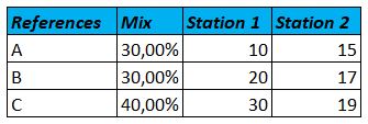
Supplier ships in sequence three references (A, B and C) manufactured on the same line. The production mix that the customer communicates to the supplier that he commits to maintain over the course of a day is 30% of A, 30% of B and 40% of C. Each reference passes through two workstations with different cycle times at each station, shown below in seconds/piece. The product passes from station 1 to station 2 and then from station 2 to the supplier conveyor.

The following image shows a schematic of the layout with the two workstations and the two operators.

The first thing the supplier does, is to identify the constraint stations depending on the reference to be manufactured, which show us that for reference A the CT (Cycle Time) is 15 seconds/part (constraint station 2), for reference B, 20 seconds/piece (constraint station 1) and for reference C 30 seconds/parte (constraint station 1), which is a bottleneck since at that rate it is unable to meet the customer demand of 25 seconds/part.

Supplier then calculates the average Cycle Time of the system to tell the customer if they are able to meet the required Takt Time. After performing the following calculation shown below he realizes that the average CT of his system is 22.5 seconds/part so they confirm to his customer that they will be able to ship at the required Takt Time.

Average Cycle Time = Mix Product A x CT Station 2 + Mix Product B x CT Station 1 + Mix Product C x CT Station 1

Average Cycle Time = 0,3 x 15 + 0,3 x 20 + 0,4 x 30

Average Cycle Time = 22.5 seconds/part

What happens on the first day of production? - The failure of the "one piece flow" system

The customer sends during the first hour the following sequence: B-B-B-B-B-B-B-B-B-A-A-A-A-A-A-A-A-A-A-A-A-A-A-A-A-A-A-A-A-A-A-C-C-C-C-C-C-C-C-C-C-C-C-C-C-C-C-C-C-C-C-C-C-C-C-C-C-C-C-C-C-C-C-C-C-C-C-C-C-C-C-C-C-C-C-C-C-C-C-C-C-C-C-C-C-C-C-C-C-C-C-C-C-C-C-C-C-C-C-C-C-C-C-C-C-C-C-C-C-C-C-C-C-C-C-C, and supplier starts to fail from sequence 58 onwards. Now we see step by step what has happened and why the calculations have failed.

Sequence is not according to the mix

A failure on the part of the supplier when calculating and telling the customer that he is able to comply with his Takt Time has been to take into account the production mix for the whole day, which is what he has committed to the customer, however there may be production peaks in which the mix is not respected even though in the daily set it is maintained. This is what has happened in this case, more C products have been ordered than calculated and supplier has not been able to supply.

Mathematical demonstration

The following has been taken into account for the calculations:

• Use of a "one piece flow" system, i.e. no stock between stations 1 and 2.
• Takt time customer = 25 seconds/part
• For the exercise it is assumed that the length of the supplier line is such that the system does not stop because the line is full.
• The calculations have been made taking into account the Cycle Time of the system, which being a one piece flow (parts are moved one at a time without stock or buffer in between) corresponds to the station with the longest cycle time depending on the reference to be manufactured.
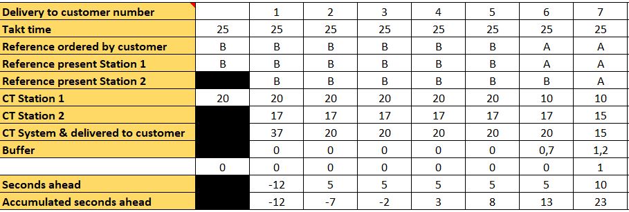
• We assume that the line is not full so the first cycle time will be the leadtime of stations 1 and 2, i.e. 20+17= 37 seconds, so our first deliveries would not meet the Takt time. This should not be a problem because usually the lines are full, but the assumption has been made like this.
• The Cycle Time of each customer delivery is calculated taking into account the maximum time between station 2 and station 1 of the previous cycle. It can be seen that in reference B, station 2 will be "starving" 3 seconds each cycle.
• Thus, we compare the cycle time of the deliveries with the Takt Time required by the customer and in this way in "Accumulated seconds ahead", we see the seconds that we are ahead or behind what the customer is requesting.
• Therefore in the first sequence delivered, which has been manufactured reference B, we have that the cycle time is marked by the station 1, with 20 seconds, which is the cycle time of the system, and that is faster than what the customer requests so we will take the customer 25-20 = 5 seconds ahead.
• In the second sequencing, a B is manufactured again, and we see that in "Accumulated seconds ahead", we have 10 seconds, because at the end of this cycle we have already taken those seconds of advantage to the customer (5 seconds of previous cycle + 5 seconds of current cycle). Below is the table with the data recorded up to the sixth sequence delivered to the customer.

• In the seventh sequence delivered, we have switched to manufacturing A products, and in this case it is station 2 that marks the cycle with 15 seconds per part, i.e. we will be getting more and more ahead of our customer.
• We have to observe here that in this case in each cycle station 1 will be "blocked" 5 seconds each cycle, this is wasted time that will never be recovered.
• It can be seen that in the sequence delivered 21, the supplier is already 158 seconds ahead of the customer.

• From the delivered sequence 22 onwards, C products are sent, whose cycle time, marked by station 1, is 30 seconds per piece, higher than the Takt Time, so that the accumulated advantage of the previous references is being lost each cycle.

• It is observed that in the sequence delivered 54, the supplier starts to fail shipments to customer (accumulated negative lead seconds), stopping its manufacturing line.

How do we solve it? - We create a buffer between stations

We can avoid or postpone in time the failure to our customer through a buffer located between station 1 and 2. The purpose of this buffer will be in this case to make independent or decoupling of stations 1 and 2.

The layout would be as shown below, and then the results of placing such a buffer would only consist of a shelf capable of storing products from station 1 to be later fed in FIFO to station 2. This will avoid the "blocked" state of station 1 when manufacturing product A, saving valuable time.

The effect of the creation of this buffer on the sequences is shown below:

• From the delivered sequences 1 to 6, there is the production of B references, in which the cycle time is set by station 1 with 20 seconds/part, and the buffer is kept empty for this reason (station 2 consumes faster than what it takes station 1 to produce) so the advantage we bring to customer is the same as in the previous case without buffer.

• From delivered sequences 7 to 21, references A are delivered in which the cycle time of station 1 is lower than that of station 2 and gives time to fill the buffer little by little. This is the interesting part of the buffer, the operator of station 1 is able to enjoy a productive time at all times, something that did not happen when the buffer was not present, and the operator had dead or waiting times (blocked).
• For the calculation of the buffer filling, the number of parts made by station 1 in the cycle time of station 2 has been taken and the unit has been subtracted by taking station 2 as a reference.
• For example in the sequence delivered number 6

Station 1 parts (manufactured during 17 seconds) = 17/10 = 1.7 parts

Station 2 parts (manufactured during 17 seconds) = 17/17 = 1 part

Difference (what is left in buffer) = 1.7 - 1 = 0.7 parts

• Subsequently all this is cumulative and is added to the result of the previous cycle as shown in the spreadsheet. As can be deduced, 0.7 parts are actually 0 parts in the buffer, a rounding down is applied.
• It is also noted that station 1 finishes manufacturing the required number of references A in the delivered sequence 15, and has already filled the buffer with 5 units. For this reason, despite the fact that station 1 is manufacturing at 30 seconds per unit (C references), station 2 is still producing units every 15 seconds, which will be the cycle time for deliveries to the customer. Since the cycle time of station 1 is now longer than that of station 2, the buffer is gradually emptying.

• In the sequence 22, products A have already finished leaving the system to move on to products C. As can be seen, since there are still parts left in the buffer, station 2 continues to set the system cycle, which is the one that removes the parts at 19 seconds/part. We have to realize that at this moment products C are already coming out, which had been made in previous sequences in station 1, taking advantage of the advantage of station 1 over station 2.

• From sequence 27 onwards, there are no more C parts in the buffer and from then on the system cycle time will be the one given by station 1, 30 seconds/part, higher than the required Takt Time of 25 seconds/part, so we are gradually losing the advantage we had over the customer until the failure that takes place in sequence 67.

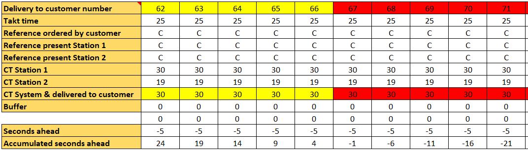
It is thus demonstrated that only by placing a buffer (a shelf) between the two stations, it is possible for station 1 to take advantage of all its productive time at the moment of manufacturing A references, which allows us in this particular case to "lengthen" 13 sequences until causing the failure in the customer. This is just an example but it goes without saying that the more A references are manufactured, the more quantity there will be in the buffer and the more capacity to cushion possible production peaks. These 13 sequences can mean stopping or not stopping on many occasions.

List of post published related to Theory of Constraints

Below you can access to all the post published related to the Theory of Constraints:

Theory of Constraints - TOC - Introduction

Identifying the constraint - TOC

Exploiting the Constraint - TOC

Subordinating everything else to the constraint - TOC

Elevating the constraint - TOC

Process optimization for manufacturing in sequence: Buffers